NBA lineups Analysis
Importing, cleaning, and PCA on NBA lineups
Background of overall project
This is the beginning in a series of NBA related analyses. Over the past fifteen years, the world of basketball has caught the wake of the analytical wave that struck baseball in the late nineties, beginning with the Oakland A’s infamous 2002 roster built with “sabermetrics”. There are a myriad of ways in which the further development might proceed. Thus far, upbraiding the conception of positions in basketball – the modern conception of “positionless” basketball – is one of the more salient results, along with the understanding of the efficiency of offenses built around the three point show considering it’s relatively larger expected value (when compared to every shot that is not a dunk/uncontested layup). Within the series, I hope to approach questions such as:
- How many different kinds of lineups (unique lineup types) are there?
- How many games/minutes/mpg are necessary to properly estimate the effectiveness of a lineup?
- To what degree do individual players’ stats correlate with the stats of lineups they are a part of?
- At what thresholds (if any) of “career minutes played” are there discrete jumps in long-term injury incidence?
- Is the injury prevalence in a season affected more by “net minutes within a time window”or “net minutes since season began”?
Loading libraries and importing data
library(tidyverse)
library(jsonlite)
library(ggplot2)
Next we need to actually import some data. This is from the nba.com lineups stat page
nba_lineups_test <- fromJSON("~/Documents/Analyses/nba_lineups_response", flatten=F)

NBA_lineups_20_21 <- nba_lineups_test$resultSets$rowSet %>% .[[1]] %>% as_tibble()

colnames(NBA_lineups_20_21) <- nba_lineups_test$resultSets$headers %>% .[[1]]

NBA_lineups_20_21[,6:49] <- lapply(NBA_lineups_20_21[,6:49], as.numeric)
We are nearly done. Notice that if we take a glance at the tibble now, some of the columns have the string “RANK” in them.
str(NBA_lineups_20_21)
## tibble [2,000 × 49] (S3: tbl_df/tbl/data.frame)
##  $ GROUP_SET        : chr [1:2000] "Lineups" "Lineups" "Lineups" "Lineups" ...
##  $ GROUP_ID         : chr [1:2000] "-101108-203109-1626164-1628969-1629028-" "-201980-202699-203552-203954-1627732-" "-202339-203500-1627742-1628366-1629627-" "-201144-202711-203497-1626220-1628378-" ...
##  $ GROUP_NAME       : chr [1:2000] "C. Paul - J. Crowder - D. Booker - M. Bridges - D. Ayton" "D. Green - T. Harris - S. Curry - J. Embiid - B. Simmons" "E. Bledsoe - S. Adams - B. Ingram - L. Ball - Z. Williamson" "M. Conley - B. Bogdanovic - R. Gobert - R. O'Neale - D. Mitchell" ...
##  $ TEAM_ID          : chr [1:2000] "1610612756" "1610612755" "1610612740" "1610612762" ...
##  $ TEAM_ABBREVIATION: chr [1:2000] "PHX" "PHI" "NOP" "UTA" ...
##  $ GP               : num [1:2000] 52 32 41 41 41 45 35 32 40 23 ...
##  $ W                : num [1:2000] 38 27 17 29 25 31 19 15 20 12 ...
##  $ L                : num [1:2000] 14 5 24 12 16 14 16 17 20 11 ...
##  $ W_PCT            : num [1:2000] 0.731 0.844 0.415 0.707 0.61 0.689 0.543 0.469 0.5 0.522 ...
##  $ MIN              : num [1:2000] 706 656 610 593 554 508 457 425 404 395 ...
##  $ E_OFF_RATING     : num [1:2000] 117 117 116 115 108 ...
##  $ OFF_RATING       : num [1:2000] 116 118 116 114 109 ...
##  $ E_DEF_RATING     : num [1:2000] 111 103 114 103 112 ...
##  $ DEF_RATING       : num [1:2000] 111 104 114 103 114 ...
##  $ E_NET_RATING     : num [1:2000] 6.5 13.9 1.8 11.9 -3.5 7.2 8.1 6.8 7.7 1 ...
##  $ NET_RATING       : num [1:2000] 4.7 14 2 10.8 -4.6 8.7 8.7 7.2 7.6 1.9 ...
##  $ AST_PCT          : num [1:2000] 0.633 0.609 0.644 0.557 0.55 0.605 0.604 0.6 0.569 0.535 ...
##  $ AST_TO           : num [1:2000] 2.42 2.02 2.17 1.7 1.65 2.07 2.28 2.46 2.14 1.58 ...
##  $ AST_RATIO        : num [1:2000] 20.3 19 20.4 16.6 16.8 19.9 19 20 18.4 16.3 ...
##  $ OREB_PCT         : num [1:2000] 0.217 0.217 0.3 0.276 0.246 0.23 0.268 0.26 0.247 0.296 ...
##  $ DREB_PCT         : num [1:2000] 0.748 0.76 0.755 0.736 0.734 0.806 0.787 0.774 0.713 0.778 ...
##  $ REB_PCT          : num [1:2000] 0.49 0.507 0.532 0.524 0.489 0.526 0.532 0.517 0.489 0.545 ...
##  $ TM_TOV_PCT       : num [1:2000] 0.115 0.127 0.134 0.133 0.137 0.132 0.116 0.114 0.117 0.142 ...
##  $ EFG_PCT          : num [1:2000] 0.579 0.579 0.571 0.558 0.543 0.598 0.55 0.596 0.585 0.508 ...
##  $ TS_PCT           : num [1:2000] 0.611 0.621 0.59 0.592 0.57 0.619 0.582 0.611 0.623 0.532 ...
##  $ E_PACE           : num [1:2000] 99.7 100.9 100 99.5 98.7 ...
##  $ PACE             : num [1:2000] 100.1 100.6 100.3 99.9 97.3 ...
##  $ PACE_PER40       : num [1:2000] 83.4 83.8 83.6 83.2 81.1 ...
##  $ POSS             : num [1:2000] 1475 1384 1279 1232 1124 ...
##  $ PIE              : num [1:2000] 0.537 0.589 0.528 0.558 0.454 0.559 0.536 0.526 0.544 0.509 ...
##  $ GP_RANK          : num [1:2000] 1 13 4 4 4 2 10 13 7 33 ...
##  $ W_RANK           : num [1:2000] 1 5 18 4 7 3 14 27 13 46 ...
##  $ L_RANK           : num [1:2000] 14814 14449 14821 14798 14817 ...
##  $ W_PCT_RANK       : num [1:2000] 5169 4837 7677 5225 5817 ...
##  $ MIN_RANK         : num [1:2000] 1 2 3 4 5 6 7 8 9 10 ...
##  $ OFF_RATING_RANK  : num [1:2000] 5131 4871 5135 5373 5927 ...
##  $ DEF_RATING_RANK  : num [1:2000] 8599 7837 8835 7808 8817 ...
##  $ NET_RATING_RANK  : num [1:2000] 6008 5227 6182 5486 8045 ...
##  $ AST_PCT_RANK     : num [1:2000] 5717 5948 5605 6616 6712 ...
##  $ AST_TO_RANK      : num [1:2000] 1725 1973 1910 3165 3282 ...
##  $ AST_RATIO_RANK   : num [1:2000] 4037 5162 4026 6819 6059 ...
##  $ OREB_PCT_RANK    : num [1:2000] 6441 6442 4800 5189 6141 ...
##  $ DREB_PCT_RANK    : num [1:2000] 7102 6341 6367 7175 7181 ...
##  $ REB_PCT_RANK     : num [1:2000] 7845 5582 5179 5321 7855 ...
##  $ TM_TOV_PCT_RANK  : num [1:2000] 8278 8798 9003 8897 9076 ...
##  $ EFG_PCT_RANK     : num [1:2000] 5222 5223 5427 5655 5931 ...
##  $ TS_PCT_RANK      : num [1:2000] 5495 5250 5991 5944 6485 ...
##  $ PACE_RANK        : num [1:2000] 10107 9891 10002 10200 11262 ...
##  $ PIE_RANK         : num [1:2000] 6119 5229 6270 5728 7600 ...
This is because they are the ranks for each lineup (each row) in that particular category (e.g. NBA_lineups_20_21[5,31] would return the rank of the number of games played by the fifth lineup on the list). These are hidden helper columns for the table for the use of sorting on the NBA’s website. We don’t want to include any of these in our analyses, so we simply cut off the columns 31 to 44. Note that we don’t want to include the first columns in our analyses, as they are just team/player identifiers, but we don’t want to remove them for the data set as they will be useful going forward. Thus for our analyses we will usually pass in NBA_lineups_20_21[,6:30] to focus on solely the columns we want.
NBA_lineups_20_21 <- NBA_lineups_20_21[,1:30]
Another consideration is the sample size here, and this is an ambiguous referent at the moment. Each lineup is itself a sample (of that lineup’s performance), but the data set as a whole is a list of lineups as well, which is of course a sample. If we look at the minimum number of games played and minutes for lineups in our dataset, we get:
min(NBA_lineups_20_21[,"GP"])
## [1] 1
min(NBA_lineups_20_21[,"MIN"])
## [1] 11
one game played and 11 minutes played respectively. In order to have only lineups that got a reasonable amount of time together, and a reasonable amount of samples taken from it, we will restrict our analysis to lineups with at least 10 games played (more than 10% of the NBA’s 2020-2021 72 game season, the non-COVID reduced season length being 82 games) and having played at least 60 minutes together (an average of half a quarter per game on a 10 games played minimum). This may seem like not many minutes, but having the same 5 players together for more than half a quarter is not altogether common for lineups that are not starting lineups. Note that our game cutoff is not a nice 30 after which we could reasonably expect the sample to be normally distributed thanks to the central limit theorem, but to see just how uncommon it was last season for a lineup to play 30 games together we can run a filter command with preserve set to true so that we aren’t replacing the underlying tibble.
NBA_lineups_20_21 %>% filter(GP>29, preserve=TRUE)
## # A tibble: 15 × 30
##    GROUP_SET GROUP_ID   GROUP_NAME    TEAM_ID TEAM_ABBREVIATI…    GP     W     L
##    <chr>     <chr>      <chr>         <chr>   <chr>            <dbl> <dbl> <dbl>
##  1 Lineups   -101108-2… C. Paul - J.… 161061… PHX                 52    38    14
##  2 Lineups   -201980-2… D. Green - T… 161061… PHI                 32    27     5
##  3 Lineups   -202339-2… E. Bledsoe -… 161061… NOP                 41    17    24
##  4 Lineups   -201144-2… M. Conley - … 161061… UTA                 41    29    12
##  5 Lineups   -203457-2… N. Noel - R.… 161061… NYK                 41    25    16
##  6 Lineups   -201572-2… B. Lopez - J… 161061… MIL                 45    31    14
##  7 Lineups   -202685-2… J. Valanciun… 161061… MEM                 35    19    16
##  8 Lineups   -203084-1… H. Barnes - … 161061… SAC                 32    15    17
##  9 Lineups   -203084-1… H. Barnes - … 161061… SAC                 40    20    20
## 10 Lineups   -201144-2… M. Conley - … 161061… UTA                 34    23    11
## 11 Lineups   -202324-2… D. Favors - … 161061… UTA                 45    33    12
## 12 Lineups   -202324-2… D. Favors - … 161061… UTA                 36    24    12
## 13 Lineups   -203109-1… J. Crowder -… 161061… PHX                 37    27    10
## 14 Lineups   -202324-2… D. Favors - … 161061… UTA                 34    23    11
## 15 Lineups   -202324-2… D. Favors - … 161061… UTA                 30    21     9
## # … with 22 more variables: W_PCT <dbl>, MIN <dbl>, E_OFF_RATING <dbl>,
## #   OFF_RATING <dbl>, E_DEF_RATING <dbl>, DEF_RATING <dbl>, E_NET_RATING <dbl>,
## #   NET_RATING <dbl>, AST_PCT <dbl>, AST_TO <dbl>, AST_RATIO <dbl>,
## #   OREB_PCT <dbl>, DREB_PCT <dbl>, REB_PCT <dbl>, TM_TOV_PCT <dbl>,
## #   EFG_PCT <dbl>, TS_PCT <dbl>, E_PACE <dbl>, PACE <dbl>, PACE_PER40 <dbl>,
## #   POSS <dbl>, PIE <dbl>
NBA_lineups_20_21 %>% filter(GP>29, preserve=TRUE) %>% count(TEAM_ABBREVIATION)
## # A tibble: 8 × 2
##   TEAM_ABBREVIATION     n
##   <chr>             <int>
## 1 MEM                   1
## 2 MIL                   1
## 3 NOP                   1
## 4 NYK                   1
## 5 PHI                   1
## 6 PHX                   2
## 7 SAC                   2
## 8 UTA                   6
NBA_lineups_20_21 %>% filter(GP>29, preserve=TRUE) %>% count(TEAM_ABBREVIATION) %>% nrow()
## [1] 8
We see that only 15 linueps played more than 30 games. Not only that, but the 15 lineups come from a total of 8 unique teams, and one team (Utah Jazz) had over a third of such lineups. So let’s apply the restrictions of at least 10 games played and at least 60 minutes played. After that we should be ready to begin the principal component analysis and variable selection.
NBA_lineups_20_21 <- NBA_lineups_20_21 %>% filter(GP >= 10 & MIN > 60)
NBA_lineups_20_21[,c("GP","MIN")] %>% summary()
##        GP             MIN
##  Min.   :10.00   Min.   : 61.0
##  1st Qu.:12.00   1st Qu.: 80.0
##  Median :16.00   Median :110.0
##  Mean   :18.56   Mean   :156.8
##  3rd Qu.:22.25   3rd Qu.:188.8
##  Max.   :52.00   Max.   :706.0
NBA_lineups_20_21 %>% str(list.len=0)
## tibble [140 × 30] (S3: tbl_df/tbl/data.frame)
##   [list output truncated]
The minimum for both GP and MIN math the filter we applied, and we see our resulting dataset has 140 entries.
Beginning the principal component analysis
Now that we have the data into a tibble, we can run a principle component analysis. PCA is a method for variable selection. Each principle component is a linear combination of the n variables in an m * n matrix. The principle components are created so that each successive principal component accounts for a smaller proportion of the explained variance (i.e. PC1 accounts for the most, PC2 the second, etc.).
NBA_lineups_20_21_pc <- prcomp(NBA_lineups_20_21[,6:30],
                               center=TRUE,
                               scale. = TRUE)
Note the
scale. = TRUE
argument here scales the data to all be unit vector. This is important in data sets where scales vary from variable to variable (note some are percentagesin our data set, some are ratios, some are gross aggregates) and without such a step, the standard deviatio of each component would be exceptionally large, providing little predictive value if used in inferential applications.
Inital impression of PCA
By running summary(NBA_lineups_20_21_pc) we can glean some cursory information.
summary(NBA_lineups_20_21_pc)
## Importance of components:
##                           PC1    PC2    PC3    PC4     PC5    PC6     PC7
## Standard deviation     2.7168 1.9882 1.9566 1.5891 1.41812 1.2369 1.14715
## Proportion of Variance 0.2952 0.1581 0.1531 0.1010 0.08044 0.0612 0.05264
## Cumulative Proportion  0.2952 0.4533 0.6065 0.7075 0.78792 0.8491 0.90176
##                            PC8     PC9    PC10    PC11    PC12    PC13    PC14
## Standard deviation     0.96393 0.76670 0.69664 0.33773 0.30117 0.29746 0.23405
## Proportion of Variance 0.03717 0.02351 0.01941 0.00456 0.00363 0.00354 0.00219
## Cumulative Proportion  0.93892 0.96244 0.98185 0.98641 0.99004 0.99358 0.99577
##                           PC15    PC16    PC17    PC18    PC19    PC20    PC21
## Standard deviation     0.19690 0.16962 0.14598 0.10951 0.06504 0.02141 0.01514
## Proportion of Variance 0.00155 0.00115 0.00085 0.00048 0.00017 0.00002 0.00001
## Cumulative Proportion  0.99732 0.99847 0.99932 0.99980 0.99997 0.99999 1.00000
##                            PC22     PC23      PC24      PC25
## Standard deviation     0.002541 0.002246 0.0008202 1.849e-16
## Proportion of Variance 0.000000 0.000000 0.0000000 0.000e+00
## Cumulative Proportion  1.000000 1.000000 1.0000000 1.000e+00
In the world of stats rarely are arbitrary decisions made. That being said, there are no rigid or mathematically sound heuristics for choosing the number of principal components to incorporate into a model. Recall that the goal here is for a re-dimensionalization, ideally to reduce the number of variables from 44 to a handful that explain a large proportion of the samples overall variance. We can see that only the top 10 principal components account for more than 1% of variation.
We may also plot a simple scree graph to see trends in the explained variation as the number of components increases. Note that this is part of the investigative stage of the analysis – this graph is merely to inform the analyst, not present data. As such, it is not very pretty, the process of creating well-constructed plots to convey information will come later, once the analyses are finished.
qplot(c(1:25), (NBA_lineups_20_21_pc$sdev^2/sum(NBA_lineups_20_21_pc$sdev^2))) +
        geom_line() +
        xlab("Principal Component") +
        ylab("Variance Explained") +
        ggtitle("Scree Plot For NBA Lineups Advanced Stats 2020-2021 Season") +
        ylim(0,1)
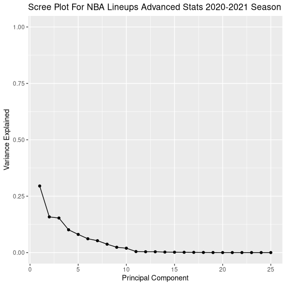
This reinforces the fact that after 10 principal components, not much more explained variance is accounted for. Thus we may safely use only the first 10 principal components in what follows.